arxiv

Where Have We Tested Gravity?

General relativity is a rich theory that makes a wide variety of experimental predictions. It’s been tested many ways, and always seems to pass with flying colors. But there’s always the possibility that a different test in a new regime will reveal some anomalous behavior, which would open the door to a revolution in our understanding of gravity. (I didn’t say it was a likely possibility, but you don’t know until you try.)

Not every experiment tests different things; sometimes one set of observations is done with a novel technique, but is actually just re-examining a physical regime that has already been well-explored. So it’s interesting to have a handle on what regimes we have already tested. For GR, that’s not such an easy question; it’s difficult to compare tests like gravitational redshift, the binary pulsar, and Big Bang nucleosynthesis.

So it’s good to see a new paper that at least takes a stab at putting it all together:

Linking Tests of Gravity On All Scales: from the Strong-Field Regime to Cosmology
Tessa Baker, Dimitrios Psaltis, Constantinos Skordis

The current effort to test General Relativity employs multiple disparate formalisms for different observables, obscuring the relations between laboratory, astrophysical and cosmological constraints. To remedy this situation, we develop a parameter space for comparing tests of gravity on all scales in the universe. In particular, we present new methods for linking cosmological large-scale structure, the Cosmic Microwave Background and gravitational waves with classic PPN tests of gravity. Diagrams of this gravitational parameter space reveal a noticeable untested regime. The untested window, which separates small-scale systems from the troubled cosmological regime, could potentially hide the onset of corrections to General Relativity.

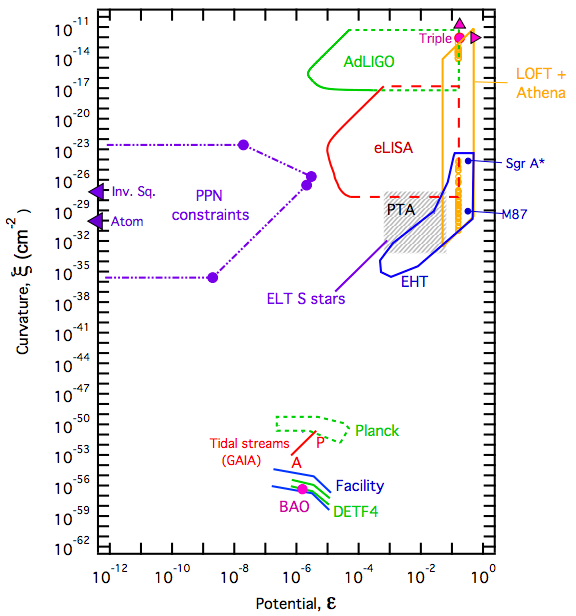
The idea is to find a simple way of characterizing different tests of GR so that they can be directly compared. This will always be something of an art as well as a science — the metric tensor has ten independent parameters (six of which are physical, given four coordinates we can choose), and there are a lot of ways they can combine together, so there’s little hope of a parameterization that is both easy to grasp and covers all bases.

Still, you can make some reasonable assumptions and see whether you make progress. Baker et al. have defined two parameters: the “Potential” ε, which roughly tells you how deep the gravitational well is, and the “Curvature” ξ, which tells you how strongly the field is changing through space. Again — these are reasonable things to look at, but not really comprehensive. Nevertheless, you can make a nice plot that shows where different experimental constraints lie in your new parameter space.

baker-etal

The nice thing is that there’s a lot of parameter space that is unexplored! You can think of this plot as a finding chart for experimenters who want to dream up new ways to test our best understanding of gravity in new regimes.

One caveat: it would be extremely surprising indeed if gravity didn’t conform to GR in these regimes. The philosophy of effective field theory gives us a very definite expectation for where our theories should break down: on length scales shorter than where we have tested the theory. It would be weird, although certainly not impossible, for a theory of gravity to work with exquisite precision in our Solar System, but break down on the scales of galaxies or cosmology. It’s not impossible, but that fact should weigh heavily in one’s personal Bayesian priors for finding new physics in this kind of regime. Just another way that Nature makes life challenging for we poor human physicists.

Where Have We Tested Gravity? Read More »

32 Comments

Planck Speaks: Bad News for Primordial Gravitational Waves?

Ever since we all heard the exciting news that the BICEP2 experiment had detected “B-mode” polarization in the cosmic microwave background — just the kind we would expect to be produced by cosmic inflation at a high energy scale — the scientific community has been waiting on pins and needles for some kind of independent confirmation, so that we could stop adding “if it holds up” every time we waxed enthusiastic about the result. And we all knew that there was just such an independent check looming, from the Planck satellite. The need for some kind of check became especially pressing when some cosmologists made a good case that the BICEP2 signal may very well have been dust in our galaxy, rather than gravitational waves from inflation (Mortonson and Seljak; Flauger, Hill, and Spergel).

Now some initial results from Planck are in … and it doesn’t look good for gravitational waves. (Warning: I am not a CMB experimentalist or data analyst, so take the below with a grain of salt, though I tried to stick close to the paper itself.)

Planck intermediate results. XXX. The angular power spectrum of polarized dust emission at intermediate and high Galactic latitudes
Planck Collaboration: R. Adam, et al.

The polarized thermal emission from Galactic dust is the main foreground present in measurements of the polarization of the cosmic microwave background (CMB) at frequencies above 100GHz. We exploit the Planck HFI polarization data from 100 to 353GHz to measure the dust angular power spectra CEE,BBℓ over the range 40<ℓ<600. These will bring new insights into interstellar dust physics and a precise determination of the level of contamination for CMB polarization experiments. We show that statistical properties of the emission can be characterized over large fractions of the sky using Cℓ. For the dust, they are well described by power laws in ℓ with exponents αEE,BB=−2.42±0.02. The amplitudes of the polarization Cℓ vary with the average brightness in a way similar to the intensity ones. The dust polarization frequency dependence is consistent with modified blackbody emission with βd=1.59 and Td=19.6K. We find a systematic ratio between the amplitudes of the Galactic B- and E-modes of 0.5. We show that even in the faintest dust-emitting regions there are no "clean" windows where primordial CMB B-mode polarization could be measured without subtraction of dust emission. Finally, we investigate the level of dust polarization in the BICEP2 experiment field. Extrapolation of the Planck 353GHz data to 150GHz gives a dust power ℓ(ℓ+1)CBBℓ/(2π) of 1.32×10⁻²μK2CMB over the 40<ℓ<120 range; the statistical uncertainty is ±0.29 and there is an additional uncertainty (+0.28,-0.24) from the extrapolation, both in the same units. This is the same magnitude as reported by BICEP2 over this ℓ range, which highlights the need for assessment of the polarized dust signal. The present uncertainties will be reduced through an ongoing, joint analysis of the Planck and BICEP2 data sets.

We can unpack that a bit, but the upshot is pretty simple: Planck has observed the whole sky, including the BICEP2 region, although not in precisely the same wavelengths. With a bit of extrapolation, however, they can use their data to estimate how big a signal should be generated by dust in our galaxy. The result fits very well with what BICEP2 actually measured. It’s not completely definitive — the Planck paper stresses over and over the need to do more analysis, especially in collaboration with the BICEP2 team — but the simplest interpretation is that BICEP2’s B-modes were caused by local contamination, not by early-universe inflation.

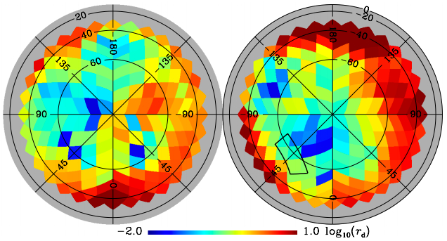
Here’s the Planck sky, color-coded by amount of B-mode polarization generated by dust, with the BICEP2 field indicated at bottom left of the right-hand circle:

planckdustmap

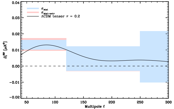
Every experiment is different, so the Planck team had to do some work to take their measurements and turn them into a prediction for what BICEP2 should have seen. Here is the sobering result, expressed (roughtly) as the expected amount of B-mode polarization as a function of angular size, with large angles on the left. (Really, the BB correlation function as a function of multipole moment.)

planck-bmode-spectrum

The light-blue rectangles are what Planck actually sees and attributes to dust. The black line is the theoretical prediction for what you would see from gravitational waves with the amplitude claimed by BICEP2. As you see, they match very well. That is: the BICEP2 signal is apparently well-explained by dust.

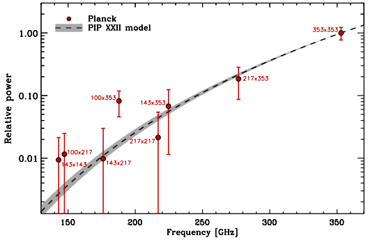
Of course, just because it could be dust doesn’t mean that it is. As one last check, the Planck team looked at how the amount of signal they saw varied as a function of the frequency of the microwaves they were observing. (BICEP2 was only able to observe at one frequency, 150 GHz.) Here’s the result, compared to a theoretical prediction for what dust should look like:

planck-dust-spectrum

Again, the data seem to be lining right up with what you would expect from dust.

It’s not completely definitive — but it’s pretty powerful. BICEP2 did indeed observe the signal that they said they observed; but the smart money right now is betting that the signal didn’t come from the early universe. There’s still work to be done, and the universe has plenty of capacity for surprising us, but for the moment we can’t claim to have gathered information from quite as early in the history of the universe as we had hoped.

Planck Speaks: Bad News for Primordial Gravitational Waves? Read More »

55 Comments

How Much Cosmic Inflation Probably Occurred?

Nothing focuses the mind like a hanging, and nothing focuses the science like an unexpected experimental result. The BICEP2 claimed discovery of gravitational waves in the cosmic microwave background — although we still don’t know whether it will hold up — has prompted cosmologists to think hard about the possibility that inflation happened at a very high energy scale. The BICEP2 paper has over 600 citations already, or more than 3/day since it was released. And hey, I’m a cosmologist! (At times.) So I am as susceptible to being prompted as anyone.

Cosmic inflation, a period of super-fast accelerated expansion in the early universe, was initially invented to help explain why the universe is so flat and smooth. (Whether this is a good motivation is another issue, one I hope to talk about soon.) In order to address these problems, the universe has to inflate by a sufficiently large amount. In particular, we have to have enough inflation so that the universe expands by a factor of more than 1022, which is about e50. Since physicists think in exponentials and logarithms, we usually just say “inflation needs to last for over 50 e-folds” for short.

So Grant Remmen, a grad student here at Caltech, and I have been considering a pretty obvious question to ask: if we assume that there was cosmic inflation, how much inflation do we actually expect to have occurred? In other words, given a certain inflationary model (some set of fields and potential energies), is it most likely that we get lots and lots of inflation, or would it be more likely to get just a little bit? Everyone who invents inflationary models is careful enough to check that their proposals allow for sufficient inflation, but that’s a bit different from asking whether it’s likely.

The result of our cogitations appeared on arxiv recently:

How Many e-Folds Should We Expect from High-Scale Inflation?
Grant N. Remmen, Sean M. Carroll

We address the issue of how many e-folds we would naturally expect if inflation occurred at an energy scale of order 1016 GeV. We use the canonical measure on trajectories in classical phase space, specialized to the case of flat universes with a single scalar field. While there is no exact analytic expression for the measure, we are able to derive conditions that determine its behavior. For a quadratic potential V(ϕ)=m2ϕ2/2 with m=2×10¹³ GeV and cutoff at MPl=2.4×10¹⁸ GeV, we find an expectation value of 2×10¹⁰ e-folds on the set of FRW trajectories. For cosine inflation V(ϕ)=Λ4[1−cos(ϕ/f)] with f=1.5×10¹⁹ GeV, we find that the expected total number of e-folds is 50, which would just satisfy the observed requirements of our own Universe; if f is larger, more than 50 e-folds are generically attained. We conclude that one should expect a large amount of inflation in large-field models and more limited inflation in small-field (hilltop) scenarios.

As should be evident, this builds on the previous paper Grant and I wrote about cosmological attractors. We have a technique for finding a measure on the space of cosmological histories, so it is natural to apply that measure to different versions of inflation. The result tells us — at least as far as the classical dynamics of inflation are concerned — how much inflation one would “naturally” expect in a given model.

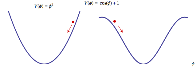
The results were interesting. For definiteness we looked at two specific simple models: quadratic inflation, where the potential for the inflaton ϕ is simply a parabola, and cosine (or “natural“) inflation, where the potential is — wait for it — a cosine. There are many models one might consider (one recent paper looks at 193 possible versions of inflation), but we weren’t trying to be comprehensive, merely illustrative. And these are two nice examples of two different kinds of potentials: “large-field” models where the potential grows without bound (or at least until you reach the Planck scale), and “small-field” models where the inflaton can sit near the top of a hill.

2potentials

Think for a moment about how much inflation can occur (rather than “probably does”) in these models. …

How Much Cosmic Inflation Probably Occurred? Read More »

16 Comments

Cosmological Attractors

I want to tell you about a paper I recently wrote with grad student Grant Remmen, about how much inflation we should expect to have occurred in the early universe. But that paper leans heavily on an earlier one that Grant and I wrote, about phase space and cosmological attractor solutions — one that I never got around to blogging about. So you’re going to hear about that one first! It’s pretty awesome in its own right. (Sadly “cosmological attractors” has nothing at all to do with the hypothetical notion of attractive cosmologists.)

Attractor Solutions in Scalar-Field Cosmology
Grant N. Remmen, Sean M. Carroll

Models of cosmological scalar fields often feature “attractor solutions” to which the system evolves for a wide range of initial conditions. There is some tension between this well-known fact and another well-known fact: Liouville’s theorem forbids true attractor behavior in a Hamiltonian system. In universes with vanishing spatial curvature, the field variables (\phi, \dot\phi) specify the system completely, defining an effective phase space. We investigate whether one can define a unique conserved measure on this effective phase space, showing that it exists for m2φ2 potentials and deriving conditions for its existence in more general theories. We show that apparent attractors are places where this conserved measure diverges in the (\phi, \dot\phi) variables and suggest a physical understanding of attractor behavior that is compatible with Liouville’s theorem.

This paper investigates a well-known phenomenon in inflationary cosmology: the existence of purported “attractor” solutions. There is a bit of lore that says that an inflationary scalar field might start off doing all sorts of things, but will quickly settle down to a preferred kind of evolution, known as the attractor. But that lore is nominally at odds with a mathematical theorem: in classical mechanics, closed systems never have attractor solutions! That’s because “attractor” means “many initial conditions are driven to the same condition,” while Liouville’s theorem says “a set of initial conditions maintains its volume as it evolves.” So what’s going on?

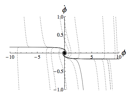
Let’s consider the simplest kind of model: you just have a single scalar field φ, and a potential energy function V(φ), in the context of an expanding universe with no other forms of matter or energy. That fully specifies the model, but then you have to specify the actual trajectory that the field takes as it evolves. Any trajectory is fixed by giving certain initial data in the form of the value of the field φ and its “velocity” \dot\phi. For a very simple potential like V(φ) ~ φ2, the trajectories look like this:
attractors

This is the “effective phase space” of the model — in a spatially flat universe (and only there), specifying φ and its velocity uniquely determines a trajectory, shown as the lines on the plot. See the dark lines that start horizontally, then spiral toward the origin? Those are the attractor solutions. Other trajectories (dashed lines) basically zoom right to the attractor, then stick nearby for the rest of their evolution. Physically, the expansion of the universe acts as a kind of friction; away from the attractor the friction is too small to matter, but once you get there friction begins to dominate and the the field rolls very slowly. So the idea is that there aren’t really that many different kinds of possible evolution; a “generic” initial condition will just snap onto the attractor and go from there.

This story seems to be in blatant contradiction with Liouville’s Theorem, which roughly says that there cannot be true attractors, because volumes in phase space (the space of initial conditions, i.e. coordinates and momenta) remain constant under time-evolution. Whereas in the picture above, volumes get squeezed to zero because every trajectory flows to the 1-dimensional attractor, and then of course eventually converges to the origin. But we know that the above plot really does show what the trajectories do, and we also know that Liouville’s theorem is correct and does apply to this situation. Our goal for the paper was to show how everything actually fits together.

Obviously (when you think about it, and know a little bit about phase space), the problem is with the coordinates on the above graph. In particular, \dot\phi might be the “velocity” of the field, but it definitely isn’t its “momentum,” in the strict mathematical sense. The canonical momentum is actually a^3\dot\phi, where a is the scale factor that measures the size of the universe. And the scale factor changes with time, so there is no simple translation between the nice plot we saw above and the “true” phase space — which should, after all, also include the scale factor itself as well as its canonical momentum.

So there are good reasons of convenience to draw the plot above, but it doesn’t really correspond to phase space. As a result, it looks like there are attractors, although there really aren’t — at least not by the strict mathematical definition. It’s just a convenient, though possibly misleading, nomenclature used by cosmologists.

Still, there is something physically relevant about these cosmological attractors (which we will still call “attractors” even if they don’t match the technical definition). If it’s not “trajectories in phase space focus onto them,” what is it? To investigate this, Grant and I turned to a formalism for defining the measure on the space of trajectories (rather than just points in phase space), originally studied by Gibbons, Hawking, and Stewart and further investigated by Heywood Tam and me a couple of years ago.

The interesting thing about the “GHS measure” on the space of trajectories is that it diverges — becomes infinitely big — for cosmologies that are spatially flat. That is, almost all universes are spatially flat — if you were to pick a homogeneous and isotropic cosmology out of a hat, it would have zero spatial curvature with probability unity. (Which means that the flatness problem you were taught as a young cosmologist is just a sad misunderstanding — more about that later in another post.) That’s fine, but it makes it mathematically tricky to study those flat universes, since the measure is infinity there. Heywood and I proposed a way to regulate this infinity to get a finite answer, but that was a mistake on our part — upon further review, our regularization was not invariant under time-evolution, as it should have been.

That left an open problem — what is the correct measure on the space of flat universes? This is what Grant and I tackled, and basically solved. Long story short, we studied the necessary and sufficient conditions for there to be the right kind of measure on the effective phase space shown in the plot above, and argued that such a measure (1) exists, and (2) is apparently unique, at least in the simple case of a quadratic potential (and probably more generally). That is, we basically reverse-engineered the measure from the requirement that Liouville’s theorem be obeyed!

So there is such a measure, but it’s very different from the naïve “graph-paper measure” that one is tempted to use for the effective phase space plotted above. (A temptation to which almost everyone in the field gives in.) Unsurprisingly, the measure blows up on the attractor, and near the origin. That is, what looks like an attractor when you plot it in these coordinates is really a sign that the density of trajectories grows very large there — which is the least surprising thing in the world, really.

At the end of the day, despite the fact that we mildly scold fellow cosmologists for their sloppy use of the word “attractor,” the physical insights connected to this idea go through essentially unaltered. The field and its velocity are the variables that are most readily observable (or describable) by us, and in terms of these variables the apparent attractor behavior is definitely there. The real usefulness of our paper would come when we wanted to actually use the measure we constructed, for example to calculate the expected amount of inflation in a given model — which is what we did in our more recent paper, to be described later.

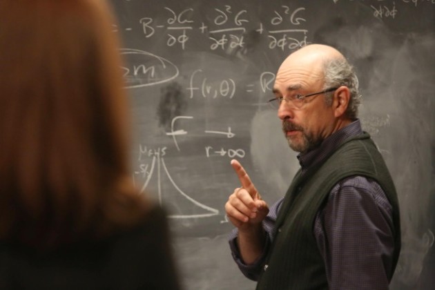
This paper, by the way, was one from which I took equations for the blackboards in an episode of Bones. It was fun to hear Richard Schiff, famous as Toby from The West Wing, play a physicist who explains his alibi by saying “I was constructing an invariant measure on the phase space of cosmological spacetimes.” 
richard-schiff-on-bones

The episode itself is great, you should watch it if you can. But I warn you — you will cry.
Cosmological Attractors Read More »

18 Comments

Single Superfield Inflation: The Trailer

This is amazing. (Via Bob McNees and Michael Nielsen on Twitter.)

Single Superfield Inflation

Backstory for the puzzled: here is a nice paper that came out last month, on inflation in supergravity.

Inflation in Supergravity with a Single Chiral Superfield
Sergei V. Ketov, Takahiro Terada

We propose new supergravity models describing chaotic Linde- and Starobinsky-like inflation in terms of a single chiral superfield. The key ideas to obtain a positive vacuum energy during large field inflation are (i) stabilization of the real or imaginary partner of the inflaton by modifying a Kahler potential, and (ii) use of the crossing terms in the scalar potential originating from a polynomial superpotential. Our inflationary models are constructed by starting from the minimal Kahler potential with a shift symmetry, and are extended to the no-scale case. Our methods can be applied to more general inflationary models in supergravity with only one chiral superfield.

Supergravity is simply the supersymmetric version of Einstein’s general theory of relativity, but unlike GR (where you can consider just about any old collection of fields to be the “source” of gravity), the constraints of supersymmetry place quite specific requirements on what counts as the “stuff” that creates the gravity. In particular, the allowed stuff comes in the form of “superfields,” which are combinations of boson and fermion fields. So if you want to have inflation within supergravity (which is a very natural thing to want), you have to do a bit of exploring around within the allowed set of superfields to get everything to work. Renata Kallosh and Andrei Linde, for example, have been examining this problem for quite some time.

What Ketov and Terada have managed to do is boil the necessary ingredients down to a minimal amount: just a single superfield. Very nice, and worth celebrating. So why not make a movie-like trailer to help generate a bit of buzz?

Which is just what Takahiro Terada, a PhD student at the University of Tokyo, has done. The link to the YouTube video appeared in an unobtrusive comment in the arxiv page for the revised version of their paper. iMovie provides a template for making such trailers, so it can’t be all that hard to do — but (1) nobody else does it, so, genius, and (2) it’s a pretty awesome job, with just the right touch of humor.

I wouldn’t have paid nearly as much attention to the paper without the trailer, so: mission accomplished. Let’s see if we can’t make this a trend.

Single Superfield Inflation: The Trailer Read More »

28 Comments

Why Probability in Quantum Mechanics is Given by the Wave Function Squared

One of the most profound and mysterious principles in all of physics is the Born Rule, named after Max Born. In quantum mechanics, particles don’t have classical properties like “position” or “momentum”; rather, there is a wave function that assigns a (complex) number, called the “amplitude,” to each possible measurement outcome. The Born Rule is then very simple: it says that the probability of obtaining any possible measurement outcome is equal to the square of the corresponding amplitude. (The wave function is just the set of all the amplitudes.)

Born Rule:     \mathrm{Probability}(x) = |\mathrm{amplitude}(x)|^2.

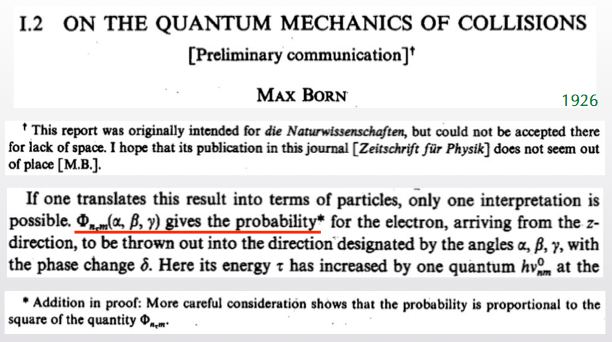
The Born Rule is certainly correct, as far as all of our experimental efforts have been able to discern. But why? Born himself kind of stumbled onto his Rule. Here is an excerpt from his 1926 paper:

Born Rule

That’s right. Born’s paper was rejected at first, and when it was later accepted by another journal, he didn’t even get the Born Rule right. At first he said the probability was equal to the amplitude, and only in an added footnote did he correct it to being the amplitude squared. And a good thing, too, since amplitudes can be negative or even imaginary!

The status of the Born Rule depends greatly on one’s preferred formulation of quantum mechanics. When we teach quantum mechanics to undergraduate physics majors, we generally give them a list of postulates that goes something like this:

  1. Quantum states are represented by wave functions, which are vectors in a mathematical space called Hilbert space.
  2. Wave functions evolve in time according to the Schrödinger equation.
  3. The act of measuring a quantum system returns a number, known as the eigenvalue of the quantity being measured.
  4. The probability of getting any particular eigenvalue is equal to the square of the amplitude for that eigenvalue.
  5. After the measurement is performed, the wave function “collapses” to a new state in which the wave function is localized precisely on the observed eigenvalue (as opposed to being in a superposition of many different possibilities).

It’s an ungainly mess, we all agree. You see that the Born Rule is simply postulated right there, as #4. Perhaps we can do better.

Of course we can do better, since “textbook quantum mechanics” is an embarrassment. There are other formulations, and you know that my own favorite is Everettian (“Many-Worlds”) quantum mechanics. (I’m sorry I was too busy to contribute to the active comment thread on that post. On the other hand, a vanishingly small percentage of the 200+ comments actually addressed the point of the article, which was that the potential for many worlds is automatically there in the wave function no matter what formulation you favor. Everett simply takes them seriously, while alternatives need to go to extra efforts to erase them. As Ted Bunn argues, Everett is just “quantum mechanics,” while collapse formulations should be called “disappearing-worlds interpretations.”)

Like the textbook formulation, Everettian quantum mechanics also comes with a list of postulates. Here it is:

  1. Quantum states are represented by wave functions, which are vectors in a mathematical space called Hilbert space.
  2. Wave functions evolve in time according to the Schrödinger equation.

That’s it! Quite a bit simpler — and the two postulates are exactly the same as the first two of the textbook approach. Everett, in other words, is claiming that all the weird stuff about “measurement” and “wave function collapse” in the conventional way of thinking about quantum mechanics isn’t something we need to add on; it comes out automatically from the formalism.

The trickiest thing to extract from the formalism is the Born Rule. That’s what Charles (“Chip”) Sebens and I tackled in our recent paper: …

Why Probability in Quantum Mechanics is Given by the Wave Function Squared Read More »

96 Comments

Galaxies That Are Too Big To Fail, But Fail Anyway

Dark matter exists, but there is still a lot we don’t know about it. Presumably it’s some kind of particle, but we don’t know how massive it is, what forces it interacts with, or how it was produced. On the other hand, there’s actually a lot we do know about the dark matter. We know how much of it there is; we know roughly where it is; we know that it’s “cold,” meaning that the average particle’s velocity is much less than the speed of light; and we know that dark matter particles don’t interact very strongly with each other. Which is quite a bit of knowledge, when you think about it.

Fortunately, astronomers are pushing forward to study how dark matter behaves as it’s scattered through the universe, and the results are interesting. We start with a very basic idea: that dark matter is cold and completely non-interacting, or at least has interactions (the strength with which dark matter particles scatter off of each other) that are too small to make any noticeable difference. This is a well-defined and predictive model: ΛCDM, which includes the cosmological constant (Λ) as well as the cold dark matter (CDM). We can compare astronomical observations to ΛCDM predictions to see if we’re on the right track.

At first blush, we are very much on the right track. Over and over again, new observations come in that match the predictions of ΛCDM. But there are still a few anomalies that bug us, especially on relatively small (galaxy-sized) scales.

One such anomaly is the “too big to fail” problem. The idea here is that we can use ΛCDM to make quantitative predictions concerning how many galaxies there should be with different masses. For example, the Milky Way is quite a big galaxy, and it has smaller satellites like the Magellanic Clouds. In ΛCDM we can predict how many such satellites there should be, and how massive they should be. For a long time we’ve known that the actual number of satellites we observe is quite a bit smaller than the number predicted — that’s the “missing satellites” problem. But this has a possible solution: we only observe satellite galaxies by seeing stars and gas in them, and maybe the halos of dark matter that would ordinarily support such galaxies get stripped of their stars and gas by interacting with the host galaxy. The too big to fail problem tries to sharpen the issue, by pointing out that some of the predicted galaxies are just so massive that there’s no way they could not have visible stars. Or, put another way: the Milky Way does have some satellites, as do other galaxies; but when we examine these smaller galaxies, they seem to have a lot less dark matter than the simulations would predict.

Still, any time you are concentrating on galaxies that are satellites of other galaxies, you rightly worry that complicated interactions between messy atoms and photons are getting in the way of the pristine elegance of the non-interacting dark matter. So we’d like to check that this purported problem exists even out “in the field,” with lonely galaxies far away from big monsters like the Milky Way.

A new paper claims that yes, there is a too-big-to-fail problem even for galaxies in the field.

Is there a “too big to fail” problem in the field?
Emmanouil Papastergis, Riccardo Giovanelli, Martha P. Haynes, Francesco Shankar

We use the Arecibo Legacy Fast ALFA (ALFALFA) 21cm survey to measure the number density of galaxies as a function of their rotational velocity, Vrot,HI (as inferred from the width of their 21cm emission line). Based on the measured velocity function we statistically connect galaxies with their host halos, via abundance matching. In a LCDM cosmology, low-velocity galaxies are expected to be hosted by halos that are significantly more massive than indicated by the measured galactic velocity; allowing lower mass halos to host ALFALFA galaxies would result in a vast overestimate of their number counts. We then seek observational verification of this predicted trend, by analyzing the kinematics of a literature sample of field dwarf galaxies. We find that galaxies with Vrot,HI<25 km/s are kinematically incompatible with their predicted LCDM host halos, in the sense that hosts are too massive to be accommodated within the measured galactic rotation curves. This issue is analogous to the "too big to fail" problem faced by the bright satellites of the Milky Way, but here it concerns extreme dwarf galaxies in the field. Consequently, solutions based on satellite-specific processes are not applicable in this context. Our result confirms the findings of previous studies based on optical survey data, and addresses a number of observational systematics present in these works. Furthermore, we point out the assumptions and uncertainties that could strongly affect our conclusions. We show that the two most important among them, namely baryonic effects on the abundances and rotation curves of halos, do not seem capable of resolving the reported discrepancy.

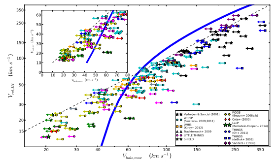
Here is the money plot from the paper:

toobigtofail

The horizontal axis is the maximum circular velocity, basically telling us the mass of the halo; the vertical axis is the observed velocity of hydrogen in the galaxy. The blue line is the prediction from ΛCDM, while the dots are observed galaxies. Now, you might think that the blue line is just a very crappy fit to the data overall. But that’s okay; the points represent upper limits in the horizontal direction, so points that lie below/to the right of the curve are fine. It’s a statistical prediction: ΛCDM is predicting how many galaxies we have at each mass, even if we don’t think we can confidently measure the mass of each individual galaxy. What we see, however, is that there are a bunch of points in the bottom left corner that are above the line. ΛCDM predicts that even the smallest galaxies in this sample should still be relatively massive (have a lot of dark matter), but that’s not what we see.

If it holds up, this result is really intriguing. ΛCDM is a nice, simple starting point for a theory of dark matter, but it’s also kind of boring. From a physicist’s point of view, it would be much more fun if dark matter particles interacted noticeably with each other. We have plenty of ideas, including some of my favorites like dark photons and dark atoms. It is very tempting to think that observed deviations from the predictions of ΛCDM are due to some interesting new physics in the dark sector.

Which is why, of course, we should be especially skeptical. Always train your doubt most strongly on those ideas that you really want to be true. Fortunately there is plenty more to be done in terms of understanding the distribution of galaxies and dark matter, so this is a very solvable problem — and a great opportunity for learning something profound about most of the matter in the universe.

Galaxies That Are Too Big To Fail, But Fail Anyway Read More »

22 Comments

Squelching Boltzmann Brains (And Maybe Eternal Inflation)

There’s no question that quantum fluctuations play a crucial role in modern cosmology, as the recent BICEP2 observations have reminded us. According to inflation, all of the structures we see in the universe, from galaxies up to superclusters and beyond, originated as tiny quantum fluctuations in the very early universe, as did the gravitational waves seen by BICEP2. But quantum fluctuations are a bit of a mixed blessing: in addition to providing an origin for density perturbations and gravitational waves (good!), they are also supposed to give rise to Boltzmann brains (bad) and eternal inflation (good or bad, depending on taste). Nobody would deny that it behooves cosmologists to understand quantum fluctuations as well as they can, especially since our theories involve mysterious aspects of physics operating at absurdly high energies.

Kim Boddy, Jason Pollack and I have been re-examining how quantum fluctuations work in cosmology, and in a new paper we’ve come to a surprising conclusion: cosmologists have been getting it wrong for decades now. In an expanding universe that has nothing in it but vacuum energy, there simply aren’t any quantum fluctuations at all. Our approach shows that the conventional understanding of inflationary perturbations gets the right answer, although the perturbations aren’t due to “fluctuations”; they’re due to an effective measurement of the quantum state of the inflaton field when the universe reheats at the end of inflation. In contrast, less empirically-grounded ideas such as Boltzmann brains and eternal inflation both rely crucially on treating fluctuations as true dynamical events, occurring in real time — and we say that’s just wrong.

All very dramatically at odds with the conventional wisdom, if we’re right. Which means, of course, that there’s always a chance we’re wrong (although we don’t think it’s a big chance). This paper is pretty conceptual, which a skeptic might take as a euphemism for “hand-waving”; we’re planning on digging into some of the mathematical details in future work, but for the time being our paper should be mostly understandable to anyone who knows undergraduate quantum mechanics. Here’s the abstract:

De Sitter Space Without Quantum Fluctuations
Kimberly K. Boddy, Sean M. Carroll, and Jason Pollack

We argue that, under certain plausible assumptions, de Sitter space settles into a quiescent vacuum in which there are no quantum fluctuations. Quantum fluctuations require time-dependent histories of out-of-equilibrium recording devices, which are absent in stationary states. For a massive scalar field in a fixed de Sitter background, the cosmic no-hair theorem implies that the state of the patch approaches the vacuum, where there are no fluctuations. We argue that an analogous conclusion holds whenever a patch of de Sitter is embedded in a larger theory with an infinite-dimensional Hilbert space, including semiclassical quantum gravity with false vacua or complementarity in theories with at least one Minkowski vacuum. This reasoning provides an escape from the Boltzmann brain problem in such theories. It also implies that vacuum states do not uptunnel to higher-energy vacua and that perturbations do not decohere while slow-roll inflation occurs, suggesting that eternal inflation is much less common than often supposed. On the other hand, if a de Sitter patch is a closed system with a finite-dimensional Hilbert space, there will be Poincaré recurrences and Boltzmann fluctuations into lower-entropy states. Our analysis does not alter the conventional understanding of the origin of density fluctuations from primordial inflation, since reheating naturally generates a high-entropy environment and leads to decoherence.

The basic idea is simple: what we call “quantum fluctuations” aren’t true, dynamical events that occur in isolated quantum systems. Rather, they are a poetic way of describing the fact that when we observe such systems, the outcomes are randomly distributed rather than deterministically predictable. …

Squelching Boltzmann Brains (And Maybe Eternal Inflation) Read More »

67 Comments

A Bit of Physics History: Ed Witten Introduces M-Theory

The Second Superstring Revolution was, like most revolutions, a somewhat messy affair, with a number of pivotal steps along the way: understanding the role of membranes in 11-dimensional supergravity, the discovery of dualities in supersymmetric gauge theories, Polchinski’s appreciation of D-branes as dynamical extended objects in string theory, and of course Maldacena’s formulation of the AdS/CFT correspondence. But perhaps the high point was Ed Witten’s formulation of M-Theory in 1995. And I just noticed that Witten sharing it with the world was captured on video.

Here is Witten’s paper:

String Theory Dynamics In Various Dimensions
Edward Witten

The strong coupling dynamics of string theories in dimension d≥4 are studied. It is argued, among other things, that eleven-dimensional supergravity arises as a low energy limit of the ten-dimensional Type IIA superstring, and that a recently conjectured duality between the heterotic string and Type IIA superstrings controls the strong coupling dynamics of the heterotic string in five, six, and seven dimensions and implies S duality for both heterotic and Type II strings.

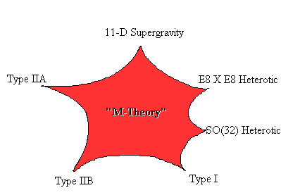
Before this result, we knew about five different kinds of string theory, each living in ten dimensions: Type I, two different Type II’s, and two different “heterotic” theories. Then there was the most symmetric form of supergravity, living in 11 dimensions, which some people thought was interesting but others thought was a curiosity that had been superseded by string theory. To everyone’s amazement, Witten showed that all of these theories are simply different limiting cases of a single underlying structure. Nobody knows what that underlying theory really is (although there are a few different formulations that work in some contexts), but we know what to call it: M-theory.

mtheory

Now Amanda Gefter, author of the new book Trespassing on Einstein’s Lawn (and a recent guest-blogger at Cocktail Party Physics), takes to Twitter to point out something I wasn’t aware of: a video record of Witten’s famous 1995 talk at USC. (I’m pretty sure this is the celebrated talk, but my confidence isn’t 100%.) [Update: folks who should know are actually saying it might be a seminar soon thereafter at Stony Brook. Witten himself admits that he’s not sure.] It’s clearly a recording by someone in the audience, but I don’t know who.

Most physics seminars are, shall we say, not all that historically exciting. But this one was recognized right away as something special. I was a postdoc at MIT at the time, and not in the audience myself, but I remember distinctly how the people who were there were buzzing about it when they returned home.

Nature giveth, and Nature taketh away. The 1995 discovery of M-theory made string theory seem more promising than ever, to the extent that just a single theory, rather than five or six. Then the 1998 discovery that the universe is accelerating made people take more seriously the idea that there might be more than one way to compactify those extra dimensions down to the four we observe — and once you have more than one, you sadly end up with a preposterously high number (the string theory landscape). So even if there is only one unifying theory of everything, there seem to be a bajillion phases it can be in, which creates an enormous difficulty in trying to relate M-theory to reality. But we won’t know unless we try, will we?

A Bit of Physics History: Ed Witten Introduces M-Theory Read More »

15 Comments

Effective Field Theory and Large-Scale Structure

Been falling behind on my favorite thing to do on the blog: post summaries of my own research papers. Back in October I submitted a paper with two Caltech colleagues, postdoc Stefan Leichenauer and grad student Jason Pollack, on the intriguing intersection of effective field theory (EFT) and cosmological large-scale structure (LSS). Now’s a good time to bring it up, as there’s a great popular-level discussion of the idea by Natalie Wolchover in Quanta.

So what is the connection between EFT and LSS? An effective field theory, as loyal readers know, an “effective field theory” is a way to describe what happens at low energies (or, equivalently, long wavelengths) without having a complete picture of what’s going on at higher energies. In particle physics, we can calculate processes in the Standard Model perfectly well without having a complete picture of grand unification or quantum gravity. It’s not that higher energies are unimportant, it’s just that all of their effects on low-energy physics can be summed up in their contributions to just a handful of measurable parameters.

In cosmology, we consider the evolution of LSS from tiny perturbations at early times to the splendor of galaxies and clusters that we see today. It’s really a story of particles — photons, atoms, dark matter particles — more than a field theory (although of course there’s an even deeper description in which everything is a field theory, but that’s far removed from cosmology). So the right tool is the Boltzmann equation — not the entropy formula that appears on his tombstone, but the equation that tells us how a distribution of particles evolves in phase space. However, the number of particles in the universe is very large indeed, so it’s the most obvious thing in the world to make an approximation by “smoothing” the particle distribution into an effective fluid. That fluid has a density and a velocity, but also has parameters like an effective speed of sound and viscosity. As Leonardo Senatore, one of the pioneers of this approach, says in Quanta, the viscosity of the universe is approximately equal to that of chocolate syrup.

So the goal of the EFT of LSS program (which is still in its infancy, although there is an important prehistory) is to derive the correct theory of the effective cosmological fluid. That is, to determine how all of the complicated churning dynamics at the scales of galaxies and clusters feeds back onto what happens at larger distances where things are relatively smooth and well-behaved. It turns out that this is more than a fun thing for theorists to spend their time with; getting the EFT right lets us describe what happens even at some length scales that are formally “nonlinear,” and therefore would conventionally be thought of as inaccessible to anything but numerical simulations. I really think it’s the way forward for comparing theoretical predictions to the wave of precision data we are blessed with in cosmology.

Here is the abstract for the paper I wrote with Stefan and Jason:

A Consistent Effective Theory of Long-Wavelength Cosmological Perturbations
Sean M. Carroll, Stefan Leichenauer, Jason Pollack

Effective field theory provides a perturbative framework to study the evolution of cosmological large-scale structure. We investigate the underpinnings of this approach, and suggest new ways to compute correlation functions of cosmological observables. We find that, in contrast with quantum field theory, the appropriate effective theory of classical cosmological perturbations involves interactions that are nonlocal in time. We describe an alternative to the usual approach of smoothing the perturbations, based on a path-integral formulation of the renormalization group equations. This technique allows for improved handling of short-distance modes that are perturbatively generated by long-distance interactions.

As useful as the EFT of LSS approach is, our own contribution is mostly on the formalism side of things. (You will search in vain for any nice plots comparing predictions to data in our paper — but do check out the references.) We try to be especially careful in establishing the foundations of the approach, and along the way we show that it’s not really a “field” theory in the conventional sense, as there are interactions that are nonlocal in time (a result also found by Carrasco, Foreman, Green, and Senatore). This is a formal worry, but doesn’t necessarily mean that the theory is badly behaved; one just has to work a bit to understand the time-dependence of the effective coupling constants.

Here is a video from a physics colloquium I gave at NYU on our paper. A colloquium is intermediate in level between a public talk and a technical seminar, so there are some heavy equations at the end but the beginning is pretty motivational. Enjoy!

Colloquium October 24th, 2013 -- Effective Field Theory and Cosmological Large-Scale Structure

Effective Field Theory and Large-Scale Structure Read More »

8 Comments
Scroll to Top